Investigating Joint- and Task-Space Impedance Controllers using Baxter Robot

Yinkai Dong^1,2, Moses C. Nah¹, Neville Hogan¹
¹MIT
²Southern University of Science and Technology

Abstract: This report investigates the implementation and comparative analysis of joint-space and task-space impedance controllers. These controllers are implemented and tested in MuJoCo simulation using a Baxter robot model. The effectiveness of these controllers is demonstrated with various tasks, e.g., tracking a predetermined trajectory in both joint- and task-spaces, sustaining a constant orientation of the end-effector, managing kinematic singularity and kinematic redundancy of the robot. For managing kinematic singularity, a comparison with operational space control was conducted.

1. Introduction

In this report, we use physics simulation software MuJoCo \citep{todorov2012mujoco} to delve deep into the application of impedance control \citep{hogan1985impedance, hogan2018impedance}. This contains a systematic exploration of joint-space and task-space impedance controllers, which are the exemplary examples. For the latter one, implementation on both position and orientation of the end-effector was conducted. With these impedance controllers, the problems of managing kinematic singularity and redundancy are discussed. For the kinematic singularity, the impedance control method was compared with operational space control \citep{khatib1985real}.

2. Impedance Control --- Theory

In this section, we briefly discuss about the theory of impedance control. Given an $n$-DOF open-chain torque-actuated robotic manipulator, the dynamics is governed by the following equations of motion \citep{murray1994mathematical,lynch2017modern}:

\[ \mathbf{M(q) \ddot{q} + C(q, \dot{q})\dot{q} + g(q) }= \boldsymbol{\tau}_{in} \] (1)

In this equation, $\mathbf{q}\in\mathbb{R}^{n}$ is a joint displacement array; $\mathbf{M(q)}\in\mathbb{R}^{n\times n}$ is the joint-space inertia matrix, which is a symmetric positive-definite matrix for all $\mathbf{q}$ \citep{murray1994mathematical,lynch2017modern}; $\mathbf{C(q, \dot{q})}\in\mathbb{R}^{n\times n}$ is the Coriolis/centrifugal matrix; $\mathbf{g(q)}\in\mathbb{R}^{n}$ is the vector of gravitational forces; $\boldsymbol{\tau}_{in}\in\mathbb{R}^n$ is the joint-torque input applied by the actuators. Throughout this report, we assume that $\mathbf{g(q)}$ is compensated, i.e., $\mathbf{g(q)}$ on the left-hand side of Eq. (1) can be neglected.

For torque-controlled robots, the goal is to determine the torque input $\boldsymbol{\tau}_{in}$ which produces desired behavior of the robot manipulator. For impedance control, two exemplary methods for designing $\boldsymbol{\tau}_{in}$ are the joint-space and task-space impedance controllers.

2.1 Joint-space Impedance Control

For the joint-space impedance control, $\boldsymbol{\tau}_{in}$ is defined by:

\[ \boldsymbol{\tau}_{in} = \mathbf{K_q(q_0-q)+B_q(\dot{q}_0-\dot{q})} \] (2)

In this equation, $\mathbf{K_q}, \mathbf{B_q} \in\mathbb{R}^{n\times n}$ are joint-space stiffness and damping matrices; $\mathbf{q}_0\in\mathbb{R}^{n}$ is the virtual joint trajectory to which the (virtual) stiffness and damping are connected.

A favorable stability property exists for this controller. If $\mathbf{K_q}, \mathbf{B_q}$ are chosen to be constant positive-definite matrices, and for a fixed $\mathbf{q}_0$, $\mathbf{q}$ asymptotically converges to $\mathbf{q}_0$ \citep{takegaki1981new, slotine1991applied}.

2.2 Task-Space Impedance Control --- Position

For the task-space impedance control, the method can be divided into controlling the position and orientation of the end-effector. For the former one, which we refer to as "position task-space impedance control," $\boldsymbol{\tau}_{in}$ is defined by:

\[ \boldsymbol{\tau}_{in} = \mathbf{ J_p(q)^{T} ( K_p (p_0 - p) + B_p (\dot{p}_0 - \dot{p}) ) } \] (3)

In this equation, $\mathbf{K_p}, \mathbf{B_p}\in\mathbb{R}^{3\times 3}$ are the translational stiffness and damping matrices; $\mathbf{p}_0\in\mathbb{R}^{3}$ is the virtual task-space trajectory to which the (virtual) stiffness and damping are connected; $\mathbf{p}=\mathbf{p}(\mathbf{q})\in\mathbb{R}^3$ is the end-effector position of the robot at joint configuration $\mathbf{q}$; $\mathbf{J_p}(\mathbf{q})\in\mathbb{R}^{3\times n}$ is the linear velocity part of the Jacobian matrix \citep{siciliano2008springer}.

As with the joint-space impedance controller (Section 2.1), a favorable stability property exists for this controller. For constant positive definite $\mathbf{K_p}, \mathbf{B_p}$ matrices, and for a constant $\mathbf{p}_0$, $\mathbf{p}$ asymptotically converges to $\mathbf{p}_0$ \citep{takegaki1981new}.

2.3 Task-Space Impedance Control --- Orientation

Along with the position task-space impedance control, orientation task-space impedance control makes the current end-effector's orientation converge to the desired orientation. In detail, given a fixed inertial frame $\{0\}$, let the current and desired orientation be denoted as ${}^{0}\mathbf{R}_{c}$ and ${}^{0}\mathbf{R}_{d}$, where ${}^{0}\mathbf{R}_{c}$ (respectively ${}^{0}\mathbf{R}_{d}$) is an element of the Special Orthogonal group SO(3) \citep{lynch2017modern,murray1994mathematical} and describes the orientation of the current (respectively desired) frame with respect to $\{0\}$.

\[ \boldsymbol{\tau}_{in} =\mathbf{J}_{\boldsymbol{\omega}}^{\mathbf{T}}(\mathbf{q})( k_\epsilon \theta \ {}^{0}\boldsymbol{\epsilon} - b_\epsilon \boldsymbol{\omega} ) \] (4)

In this equation, ${}^{0}\boldsymbol{\epsilon}\in\mathbb{R}^3$ and $\theta \in [ 0, \pi)$ correspond to the elements of the axis-angle notation \citep{lynch2017modern} of ${}^{c}\mathbf{R}_{d}={}^{0}\mathbf{R}_{c}^{T} \ {}^{0}\mathbf{R}_{d}$, respectively; superscript $0$ is used to emphasize that the axis is expressed with respect to $\{0\}$; $k_e, b_e\in\mathbb{R}$ are positive scalar values which correspond to the rotational stiffness and damping attached to axis ${}^{0}\boldsymbol{\epsilon}$, respectively; $\boldsymbol{\omega} \in \mathbb{R}^{3}$ is the angular velocity of the end-effector; $\mathbf{J}_{\boldsymbol{\omega}}(\mathbf{q})\in\mathbb{R}^{3\times n}$ is the angular velocity part of the Jacobian matrix.

2.4 Superposition Principle of Mechanical Impedances

Even though each equation of the impedance controller is a nonlinear operator, these controllers can be "linearly" superimposed \citep{hogan1985impedance}. This is the "superposition principle" of mechanical impedances, which can be expressed as:

\[ \boldsymbol{\tau}_{in} = \sum_{i=1}^{n}\boldsymbol{\tau}_{in,i} \] (5)

In this equation, $\boldsymbol{\tau}_{in,i}$ is the $i$-th impedance controller which is superimposed. While different types of impedance controllers other than Eq. (2), (3), (4) can be used, in this report we focus on using Eq. (2), (3), (4) as the basic element of the impedance controller.

The superposition principle of mechanical impedances plays a crucial role to solve multiple tasks, e.g., managing kinematic redundancy and singularity of the robotic manipulator. The details are presented in the next section.

3. Simulation with Baxter Robot

In this section, we show the implementation of multiple impedance controllers in simulation (Section 2). For the implementation, we use MuJoCo simulator \citep{todorov2012mujoco} and Baxter robot model.

3.1 Model of Baxter Robot

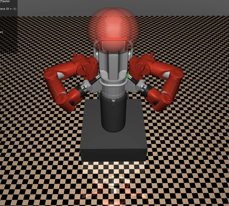
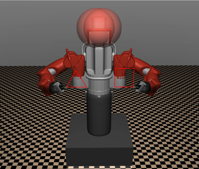
The Baxter robot, developed by Rethink Robotics is a dual-arm robot. Each arm has 7-DOF (Figure \ref{Baxter Model}). For each joint of the robot, (ideal) torque actuators are mounted. Since Baxter robot already contains a low-level gravity compensation controller, gravity was set to be a zero vector in the simulation.

MuJoCo model of Baxter Robot.

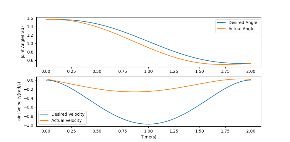
3.2 Implementation of Joint-space Impedance Control

For both arms of the Baxter robot, a joint-space impedance controller (Eq. (2)) was implemented. For the virtual joint trajectory $\mathbf{q}_0(t)$, the minimum-jerk trajectory \citep{hogan1987moving,flash1987control} was used:

\[ \mathbf{q}_0(t) = \begin{cases} \mathbf{q}_{0,i} & \text{$t(6)

Virtual trajectory and actual trajectory of the elbow-joint with joint-space impedance control. The initial joint angle for the right hand and left hand are ${\bf q}_{0, i, r}$ = [-0.314, 0.1, 1.571, 1.571, 0.393, 1.571, -1.571], ${\bf q}_{0, i, l}$ = [0.314, 0.1, -1.571, 1.571, -0.393, 1.571, 1.571]. The final joint angle for the right hand and left hand are ${\bf q}_{0, f, r}$ = [-0.105, 0.033, 0.524, 0.524, 0.131, 0.524, -0.524], ${\bf q}_{0, f, l}$ = [0.105, 0.033, -0.524, 0.524, -0.131, 0.524, 0.524]. For the plot the second wrist joint, which is the sixth joint of the right/left arm, was chosen. ${{\mathbf{K_q}}} = 50{{\mathbf{I}}_7}$, $\mathbf{B_q} = 10\mathbf{I}_7$ where $\mathbf{I}_7 \in \mathbb{R}^{7\times 7}$ is an identity matrix.

3.3 Implementation of Task-Space Impedance Control — The Problem of Kinematic Redundancy

For both arms of the Baxter robot, position task-space impedance controller (Eq. (3)) was implemented. For $\mathbf{p}_0(t)$, a circular trajectory was used:

\[ \mathbf{p}_0(t) = \begin{bmatrix} r_x \\ r_y + r_0 \cos(\omega t + \phi) \\ r_z + r_0 \sin(\omega t + \phi) \end{bmatrix} \] (7)

(a) Joint-space trajectory

(b) Cartesian position of the left hand

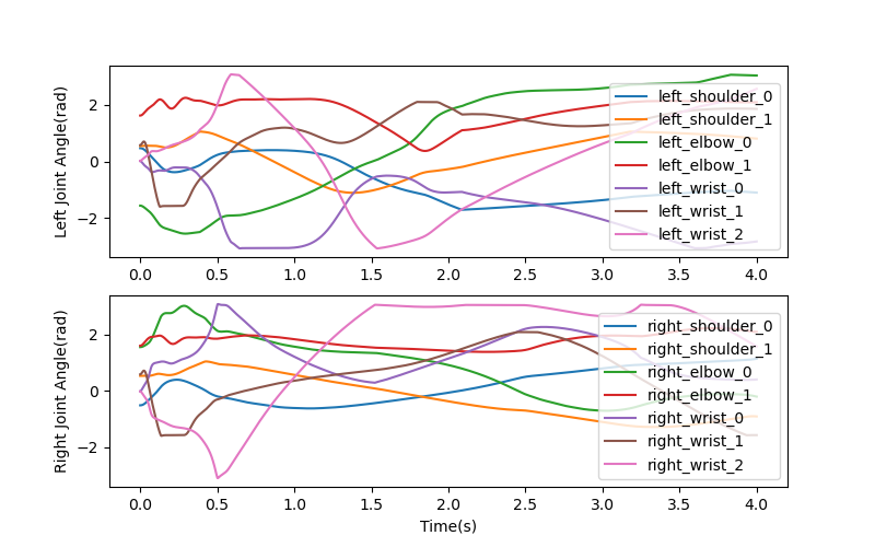
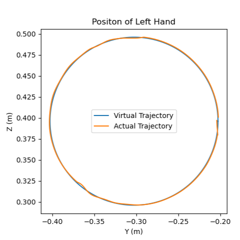
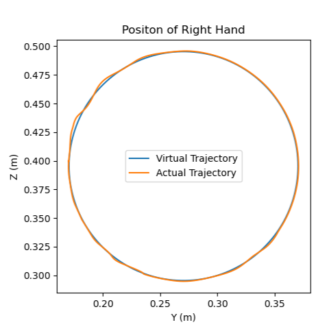
The resulting Cartesian-space trajectory of the end-effector is (almost) a circle. It is suspected that perfect tracking was not achieved due to the joint limit of the Baxter robot defined in the MuJoCo model. As shown in the joint trajectory (a), because of the kinematic redundancy of the Baxter robot, (i.e., for a 7-DOF arm with a 3-dimensional task, there is a 4-dimensional kinematic redundancy), an undesired motion in the joint-space occurs.

3.4 Managing Kinematic Redundancy with Impedance Superposition

To manage the kinematic redundancy of the robot, a joint-space impedance controller (Eq. (2)) is superimposed to the position task-space impedance controller (Eq. (3)).

(a) Joint-space trajectory

(b) Cartesian position of the left hand with superposition

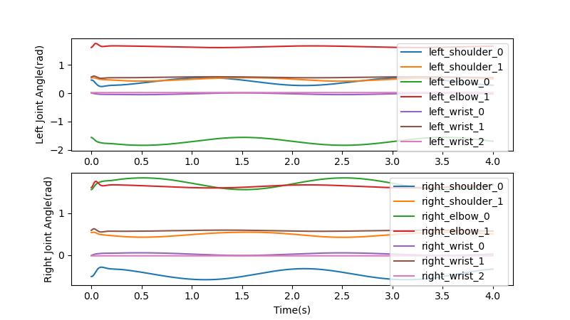
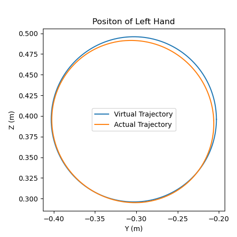
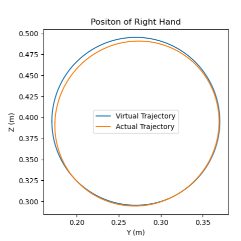
The results showed that after superimposing two impedance controllers, the angular trajectory of each joint became smoother, and the kinematic redundancy of the robot is managed. However, as shown in (b, c), task conflict exists between the two impedance controllers, which thereby increases the tracking error in Cartesian space.

3.5 Orientation Task-space Impedance Control

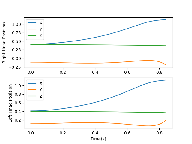
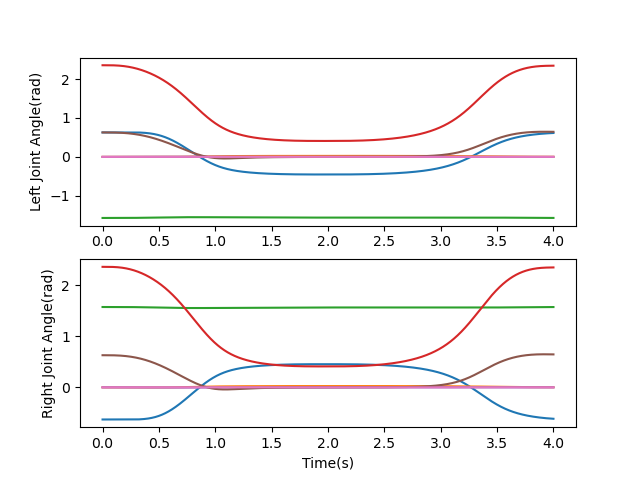
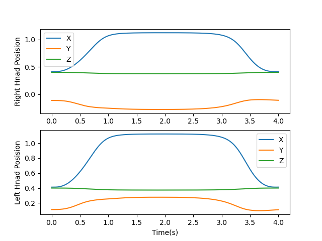
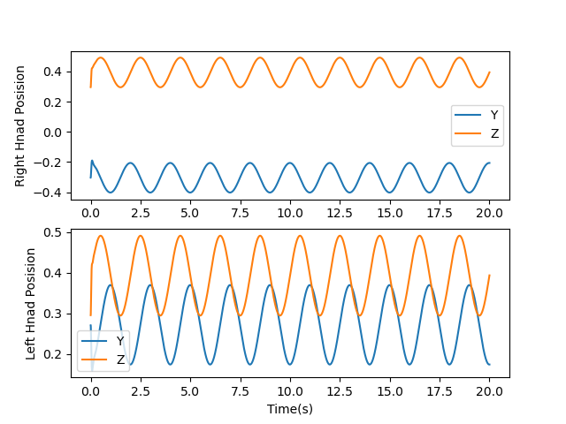
The task of tracking a task-space trajectory while maintaining a specific orientation was implemented. Each hand of the Baxter robot is given a pre-determined orientation and virtual trajectory planned in task-space, as shown below. The virtual trajectory of the right (respectively left) hand is a triangle (respectively square).

Simulation posture of Baxter Robot and the virtual task-space trajectory of both arms.

(a) Triangle trajectory results

(b) Square trajectory results

(d) Orientation error of left hand

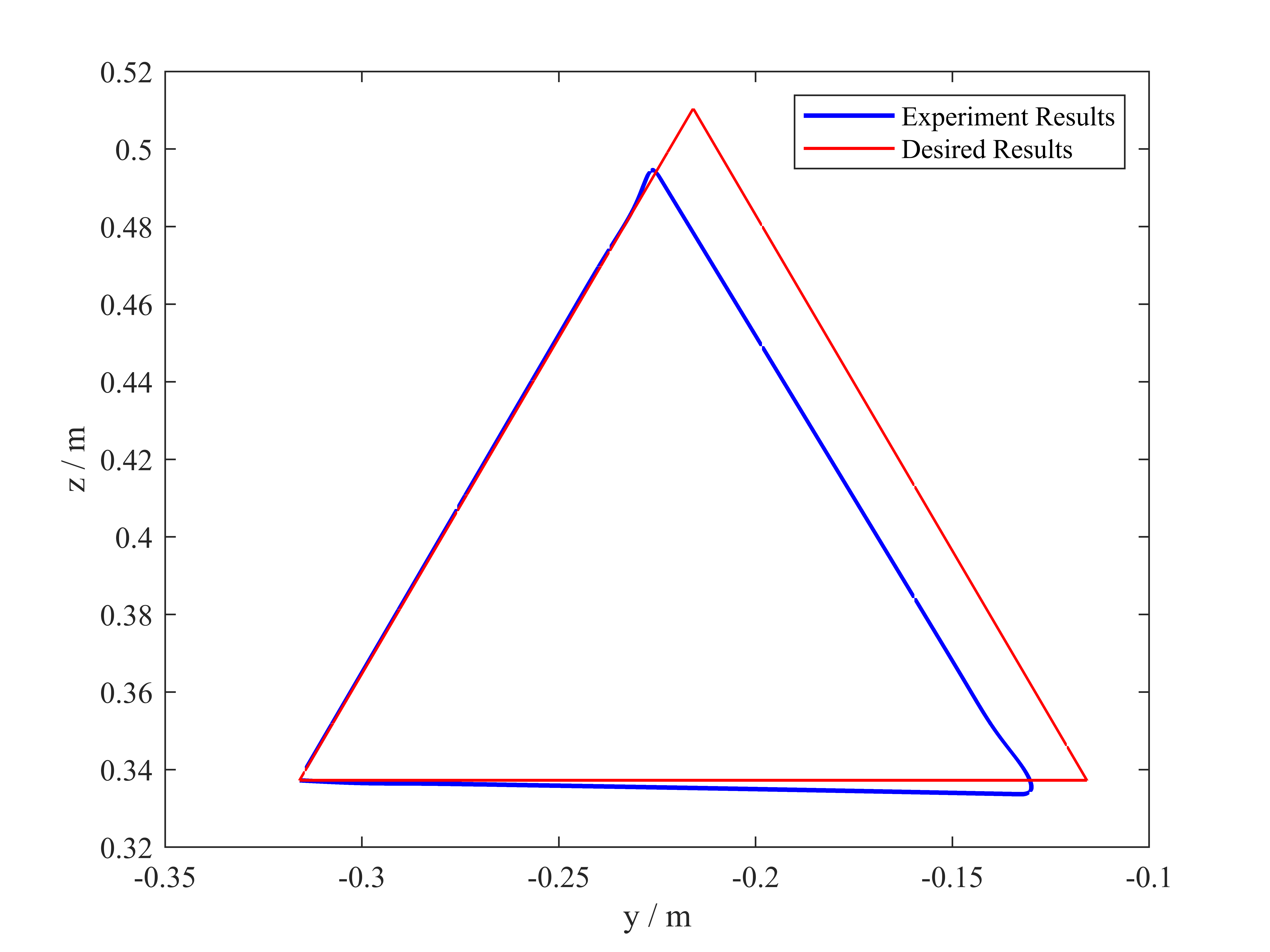
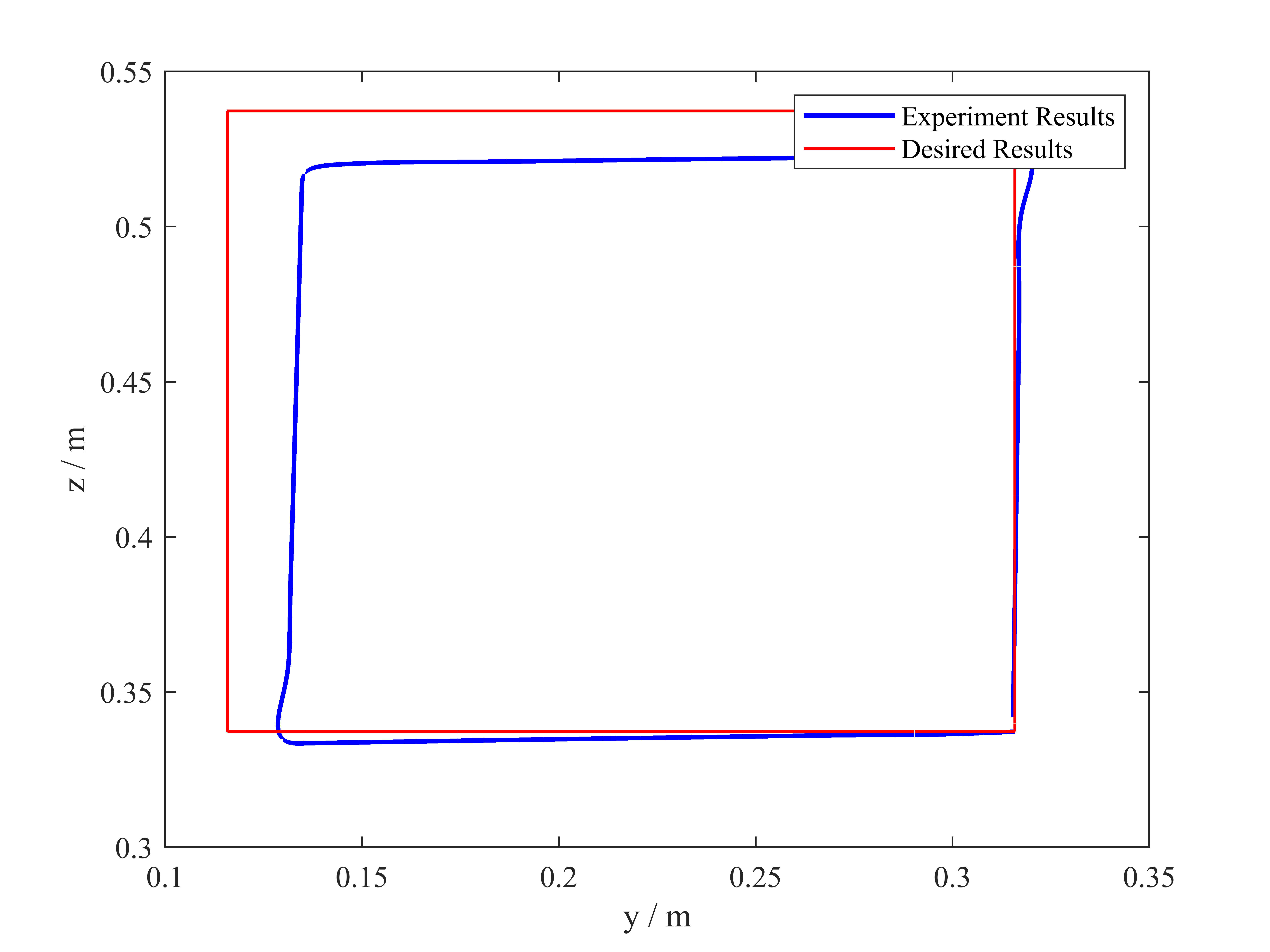
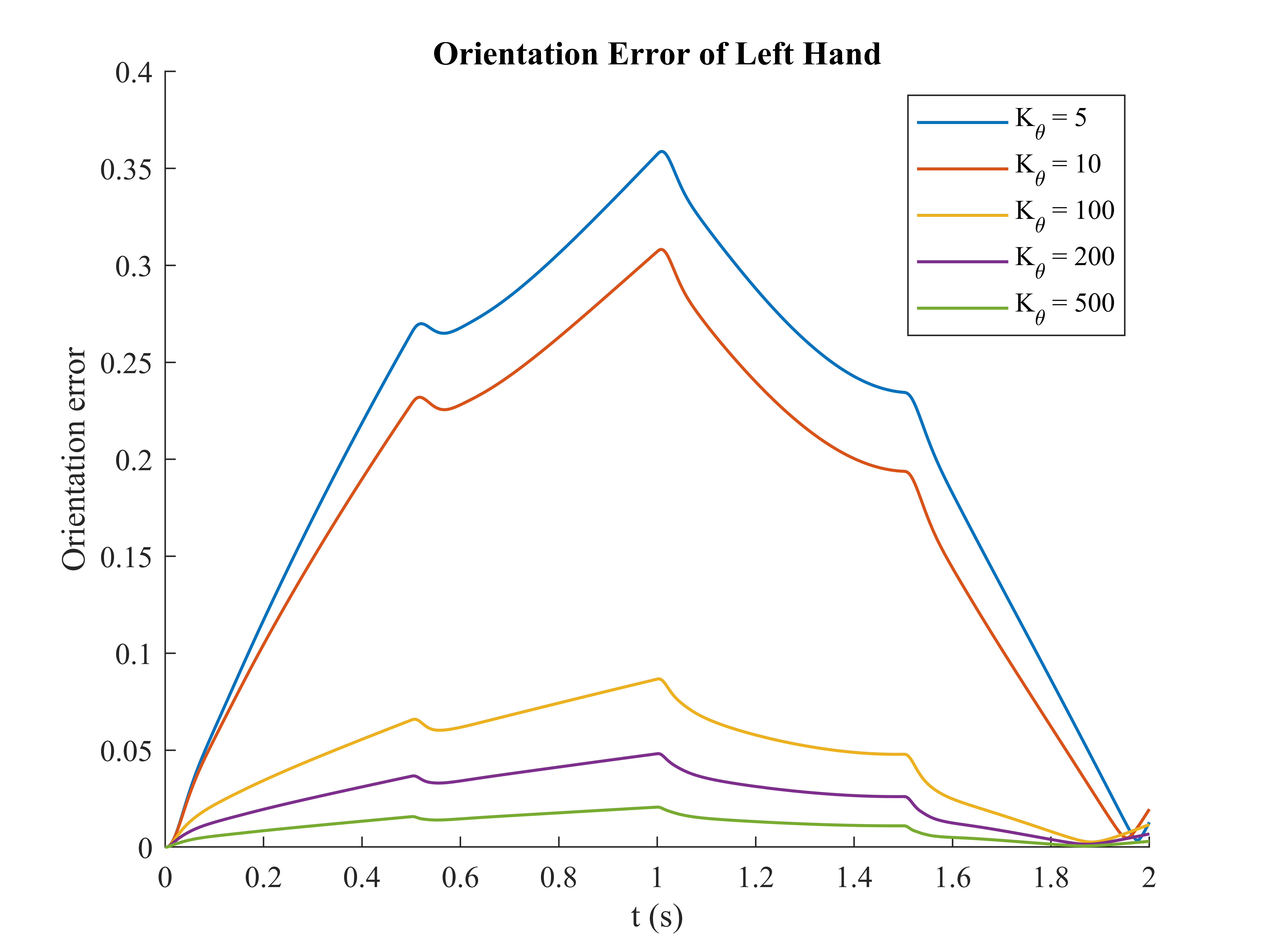
The resulting end-effector trajectory for (a) triangle and (b) square virtual trajectories. Parameters: $\mathbf{K_q} = 200{{\mathbf{I}}_7}$, $\mathbf{B_q} = 5{{\mathbf{I}}_7}$, $\mathbf{K_p} = 5 {{\mathbf{I}}_3}$, $\mathbf{B_q} = 7{{\mathbf{I}}_3}$, $ k_{\theta} = 5$, $b_{\theta} = 7$. The right-hand trajectory is represented by a triangle of length 0.2 in YZ Plane, starting at point $\mathbf{p_{0, r}} = [0.84, -0.32, 0.34] m$. The trajectory of the left hand is represented by a square of length 0.2 in YZ Plane, starting at point $\mathbf{p_{0, l}}=[0.84,0.32,0.34]m$. The initial joint angle for the right hand and left hand are: $\mathbf{q}_{0, r}$ = [-0.628, 0.524, 1.571, 1.571, 0, 0.628, 0] $rad$, $\mathbf{q}_{0, l}$ = [0.628, 0.524, -1.571, 1.571, 0, 0.628, 0] $rad$, respectively.

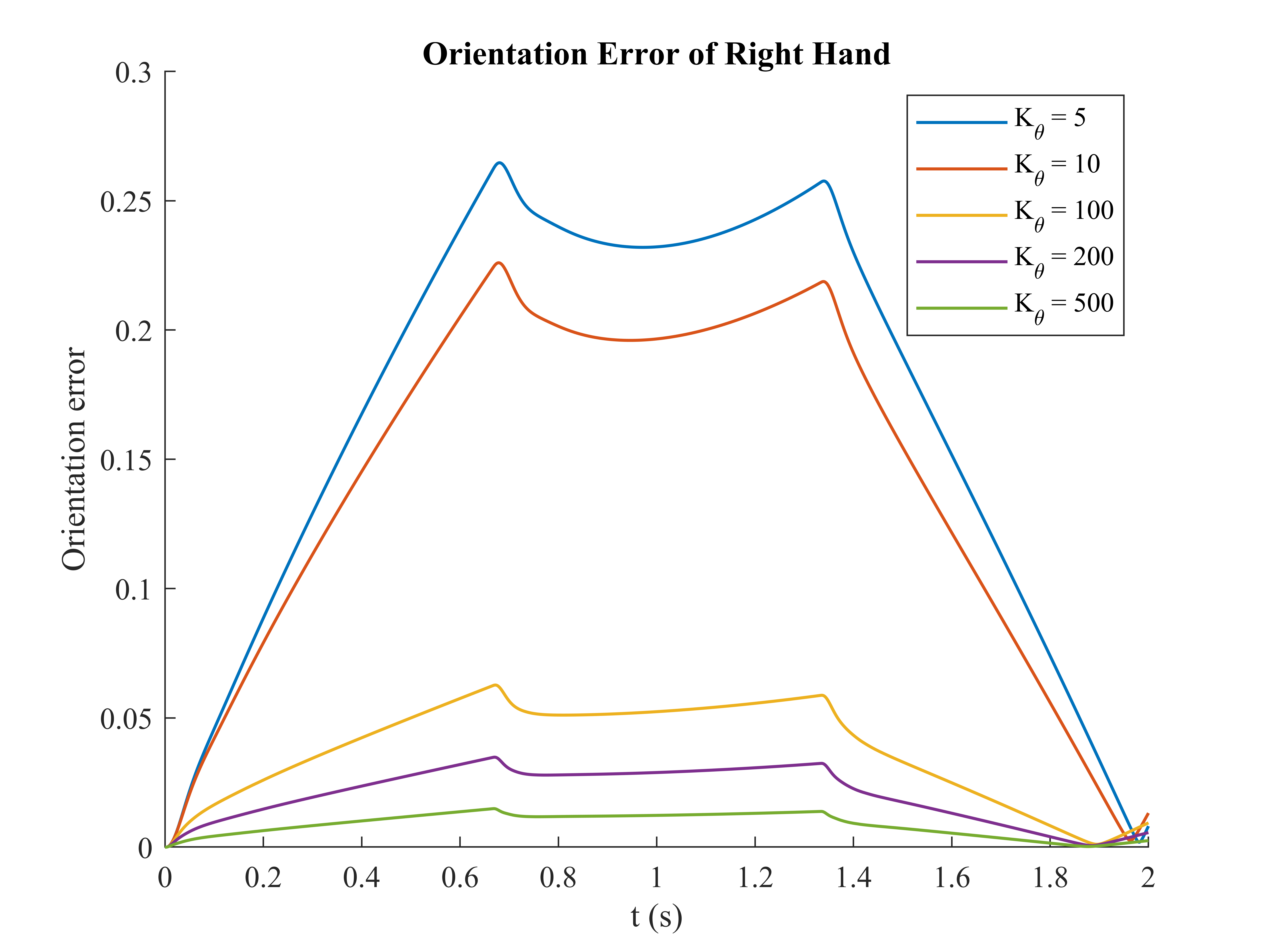
Deviations from the task-space trajectory are observed when the end-effector moves away from the initial points $\mathbf{p_{0, r}}$ and $\mathbf{p_{0, l}}$. These deviations can be attributed to the influence between virtual stiffness and damping of multiple impedance controllers. The orientation error is calculated by the Frobenius norm of the difference between the current and desired orientation matrices $\mathbf{{}^{0}R_c^{T}}~\mathbf{{}^{0}R_d}- {\bf I}_{3}$ over time. The orientation error is small when approaching the initial point $\mathbf{p_{0, r}}$ and $\mathbf{p_{0, l}}$, and as the orientation virtual stiffness $k_{\theta}$ increases, the overall error decreases.

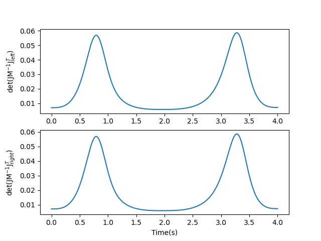
3.6 Managing Kinematic Singularity --- A Comparison with Operational Space Control

We show how the robot's behavior near kinematic singularity can be managed using impedance control. For this, a comparison of performance with Operational Space Control \citep{khatib1985real} was conducted. For the Operational Space Control, the following controller input was used \citep{khatib1985real}:

\[ \boldsymbol{\tau}_{in} = \mathbf{J}(q)^{T} \cdot \mathbf{F}_{in} \] (8)

where:

${{\bf{F}}_{in}} = {\bf{F}}_{in}^\prime + {\bf{F}}_{in}^*$
${\bf{F}}_{in}^* = {\boldsymbol \Lambda }({\bf{q}})\{ - {{\bf{b}}^*} - {\bf{\dot J}}\left( {\bf{q}} \right){\bf{\dot q}}\}$
$\boldsymbol{\Lambda}\bf(q) = (J(q) M^{-1}(q) J(q)^{T})^{-1}$
${{\bf{b}}^*} = - {\bf{J}}\left( {\bf{q}} \right){{\bf{M}}^{ - 1}}({\bf{q}}){\bf{C}}({\bf{q}},{\bf{\dot q}}){\bf{\dot q}} - {\bf{J}}\left( {\bf{q}} \right){{\bf{M}}^{ - 1}}({\bf{q}}){\bf{g}}({\bf{q}})$
${\bf{F}}_{in}^\prime = {\boldsymbol \Lambda }({\bf{q}})\{ {{{\bf{\ddot p}}}_0} + {\bf{K}_o}\left( {{{\bf{p}}_0} - {\bf{p}}} \right) + {\bf{B}}_o\left( {{{{\bf{\dot p}}}_0} - {\bf{\dot p}}} \right)\}$

In these equations, $\bf{K}_o$ is the stiffness matrix of the operational space control, $\bf{B}_o$ is the damping matrix of the operational space control, $\boldsymbol{\Lambda}\bf(q)$ is the "generalized moment of inertia" matrix \citep{asada1983geometrical}, which is the inverse of the "end-point mobility tensor" \citep{hogan1985impedance}.

We forced the robot's end-effector to reach near kinematic singularity, by controlling $\mathbf{p_0}(t)$ of the position task-space impedance controller (Eq. (3)) and operational space control (Eq. (8)). In detail, $\mathbf{p_0}(t)$ was chosen to be a minimum-jerk trajectory, and the final Cartesian position of the trajectory was set to be sufficiently outside the reachable workspace of the robot. This eventually "straightens" the robot manipulator and consequently leads to a kinematic singularity.

For Operational Space Control, when the robot's end-effector approaches near kinematic singularity (i.e., the Jacobian matrix becomes rank-deficient), the generalized moment of inertia becomes unbounded. Consequently, the control input is unbounded, which thereby causes the robot to be unstable near the kinematic singularity. This behavior is an inevitable constraint of Operational Space Control, dictated by the mathematical characteristics of the controller design.

(a) OSC Joint-space trajectory

(b) OSC end-effector Cartesian trajectory

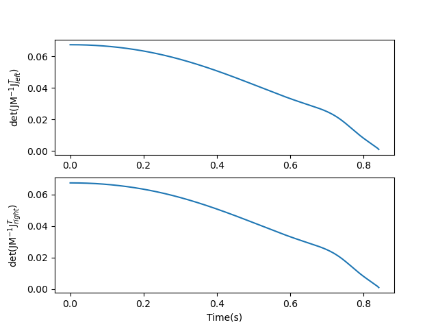
On the other hand, superimposing multiple impedance controllers manages kinematic singularity without introducing instability. This is due to the fact that an inverse of the Jacobian matrix is not required for the task-space impedance controller.

(d) Joint-space trajectory with impedance control

(e) End-effector Cartesian trajectory with impedance control

(f) Determinant of $\boldsymbol{\Lambda}^{-1}\mathbf{(q)}$ with impedance control

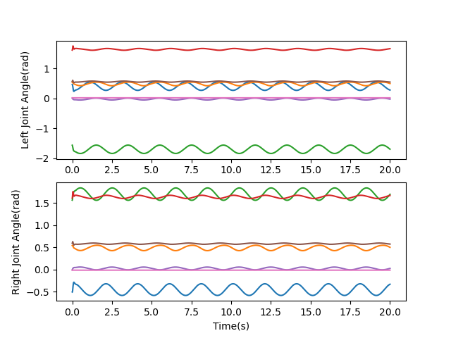
3.7 The Problem of Repeatability

For kinematically redundant robots, it is well known that the repeating motion in task-space produces a non-negligible drift in joint-space trajectories \citep{klein1983review}. In other words, given an end-effector position $\mathbf{p}$, there exists an infinite number of solutions for $\mathbf{q}$ which produce the same $\mathbf{p = f(q)}$. This problem of repeatability (or integrability) \citep{mussa1991integrable} can be addressed with impedance controller, where for a given $\mathbf{p}$, there exists a unique $\mathbf{q}$, hence the map from $\mathbf{p}$ to $\mathbf{q}$ is well-defined.

To explore the performance of repeatability using impedance control, we use the same trajectory of the position task-space impedance control in Section 3.4, Eq. (7) and repeat the circle trajectory multiple times, as shown below. The findings indicate that the robot system's motion under impedance control exhibits a high level of repeatability in both joint- and task-space trajectories.

(a) Joint-space trajectory repeatability

(b) End-effector Cartesian trajectory repeatability

4. Conclusion

In conclusion, this study presents an in-depth exploration and comparison of various impedance controllers: joint-space impedance control and task-space impedance control. Simulations using Baxter Robot demonstrate the effectiveness of these impedance controllers for multiple tasks. For instance, we show that tracking a predetermined trajectory in both joint- and task-spaces, sustaining a constant orientation of the end-effector, and managing kinematic singularity and kinematic redundancy of the robot can be achieved with impedance controllers. Overall, the findings affirm the practicality and potential of impedance controllers in multiple robotic applications.

References

Todorov, E., Erez, T., & Tassa, Y. (2012). MuJoCo: A physics engine for model-based control. In 2012 IEEE/RSJ International Conference on Intelligent Robots and Systems.
Hogan, N. (1985). Impedance control: An approach to manipulation: Part I—Theory. Journal of dynamic systems, measurement, and control.
Hogan, N. (2018). Impedance Control: An Approach to Manipulation: Part I—Theory. Journal of Dynamic Systems, Measurement, and Control.
Murray, R. M., Li, Z., Sastry, S. S., & Sastry, S. S. (1994). A mathematical introduction to robotic manipulation.
Lynch, K. M., & Park, F. C. (2017). Modern robotics.
Khatib, O. (1985). Real-time obstacle avoidance for manipulators and mobile robots.
Takegaki, M., Ito, Y., Yamaguchi, T., & Arimoto, H. (1981). New Control Scheme for Robot Manipulators: Joint Impedance Control with Adaptable Joint Stiffness and Damping.
Slotine, J.-J. E., & Li, W. (1991). Applied Nonlinear Control.
Siciliano, B., & Khatib, O. (2008). Springer Handbook of Robotics.
Hermus, J., et al. (2021). Exploiting the Superposition Principle in Mechanical Impedance Control.
Asada, H., & Slotine, J.-J. E. (1983). Geometrical Control of Robot Manipulators.
Hogan, N. (1987). Moving gracefully: Quantitative theories of motor coordination. Trends in Neurosciences.
Flash, T., & Hogan, N. (1987). The coordination of arm movements: an experimentally confirmed mathematical model. Journal of Neuroscience.
Klein, C. A., & Huang, C. C. (1983). Review of Pseudoinverse Control for Use with Kinematically Redundant Manipulators. IEEE Transactions on Systems, Man, and Cybernetics.
Mussa-Ivaldi, F. A., & Hogan, N. (1991). Integrable solutions of kinematic redundancy via impedance control. International Journal of Robotics Research.